How fine should the beamforming grid be?

A pixel pitch of \(\lambda/2\) is a common choice, but the pitch an image needs follows from its k-space support, which depends on the aperture, the steering, the bandwidth, and whether the image is RF or IQ.

In this notebook we derive the limits zea checks against, compare them to a beamformed point target, and see when \(\lambda/2\) is too coarse or needlessly fine.

 

‼️ Important: This notebook is optimized for GPU/TPU. Code execution on a CPU may be very slow.

If you are running in Colab, please enable a hardware accelerator via:

Runtime → Change runtime type → Hardware accelerator → GPU/TPU 🚀.

%%capture
%pip install zea

import os

os.environ["KERAS_BACKEND"] = "jax"
os.environ["ZEA_DISABLE_CACHE"] = "1"
os.environ["TF_CPP_MIN_LOG_LEVEL"] = "3"

import matplotlib.pyplot as plt
import numpy as np
from keras import ops
from matplotlib.patches import Rectangle
from scipy.signal import hilbert
from scipy.signal.windows import tukey

import zea
from zea import Parameters
from zea.beamform.beamformer import fnum_window_fn_tukey, fnumber_mask
from zea.beamform.delays import compute_t0_delays_planewave
from zea.beamform.pixelgrid import aliasing_limits
from zea.func import log_compress
from zea.probes import create_probe_geometry
from zea.visualize import set_mpl_style

zea.init_device(verbose=False)
set_mpl_style()

BLUE, CYAN, GREEN, RED = "#4fc3f7", "#00e5ff", "#66bb6a", "#ef5350"

zea: Using backend 'jax'

1. The k-space support of a beamformed image

A transmit along the unit vector \(\mathbf{t}\) and a receive along the unit vector \(\mathbf{r}\) at frequency \(f\) contribute the spatial frequency

\[\mathbf{k} = \frac{f}{c}\left(\mathbf{t} + \mathbf{r}\right) = \frac{\mathbf{t} + \mathbf{r}}{\lambda}\]

to the image (Walker and Trahey). Here \(\mathbf{k}\) is a vector with components \(k_x\) and \(k_z\), in cycles per metre. When \(\mathbf{t}\) and \(\mathbf{r}\) both point along \(z\), this gives \(k_z = 2/\lambda\), twice the spatial frequency of the wave itself, because a pixel \(\lambda/2\) deeper adds \(\lambda\) to the pulse-echo path. The same holds along any direction they share, and \(|\mathbf{k}|\) gets smaller the further apart they point.

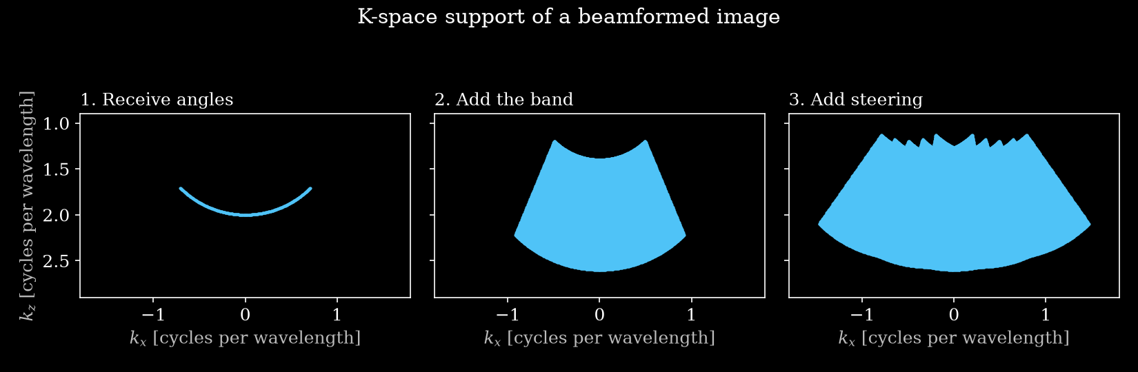
The support follows from sweeping each term:

• the receive angle over \(\tan\theta_r \le 1/(2F)\), with \(F\) the f-number

• the frequency over the band

• the transmit over the steering angles

Here is an example for a 5 MHz pulse with 3 MHz of bandwidth, \(F = 0.5\), and five plane waves up to \(\pm 25°\).

sound_speed = 1540.0
center_frequency = 5e6
bandwidth = 3e6
wavelength = sound_speed / center_frequency
f_number = 0.5
steering = np.deg2rad([-25, -12.5, 0, 12.5, 25])


def k_support(frequencies, polar_angles, f_number):
    """All k = f (t + r) / c in cycles per wavelength, with shape (n_points, 2)."""
    max_angle = np.arctan(1 / (2 * f_number))
    r = np.linspace(-max_angle, max_angle, 301)
    f, t, r = np.meshgrid(frequencies, polar_angles, r)
    k_x = f * (np.sin(t) + np.sin(r)) / sound_speed
    k_z = f * (np.cos(t) + np.cos(r)) / sound_speed
    return np.stack([k_x.ravel(), k_z.ravel()], axis=-1) * wavelength


frequencies = center_frequency + np.linspace(-0.5, 0.5, 101) * bandwidth
steps = [
    ("1. Receive angles", [center_frequency], [0.0]),
    ("2. Add the band", frequencies, [0.0]),
    ("3. Add steering", frequencies, steering),
]

fig, axes = plt.subplots(1, 3, figsize=(11, 3.6), sharex=True, sharey=True)
for ax, (title, f, t) in zip(axes, steps):
    k = k_support(f, t, f_number)
    ax.scatter(*k.T, s=4, color=BLUE, linewidths=0, rasterized=True)
    ax.set_title(title, loc="left")
    ax.set_xlabel("$k_x$ [cycles per wavelength]")
    ax.set_aspect("equal")
axes[0].set_xlim(-1.8, 1.8)
axes[0].set_ylim(2.9, 0.9)
axes[0].set_ylabel("$k_z$ [cycles per wavelength]")
fig.suptitle("K-space support of a beamformed image")
plt.tight_layout()
plt.savefig("kspace_support_build_up.png", dpi=150)
plt.close()

2. Comparison with a beamformed point target

We simulate a point scatterer with these settings and beamform it on a \(\lambda/16\) grid, so that its 2D Fourier transform shows the support. This grid is well within all the limits below, so we call the result the reference image: what a coarser grid should reproduce. The RF is band-limited to give the band known edges, and we use a smooth receive aperture instead of the default hard f-number mask, see section 5.

n_el = 192
element_pitch = wavelength / 2
probe_geometry = create_probe_geometry(n_el, element_pitch)

fine_pitch = wavelength / 16
n_grid = 513
half_extent = (n_grid - 1) / 2 * fine_pitch
depth = 10e-3
sampling_frequency = 16 * center_frequency
n_ax = 4096


def transmit_geometry(polar_angles):
    n_tx = len(polar_angles)
    return dict(
        focus_distances=np.full(n_tx, np.inf),
        probe_geometry=probe_geometry,
        tx_apodizations=np.ones((n_tx, n_el)),
        polar_angles=np.asarray(polar_angles, dtype=float),
        transmit_origins=np.zeros((n_tx, 3)),
    )


def make_parameters(polar_angles, **kwargs):
    n_tx = len(polar_angles)
    settings = dict(
        xlims=(-half_extent, half_extent),
        zlims=(depth - half_extent, depth + half_extent),
        grid_size_x=n_grid,
        grid_size_z=n_grid,
    )
    return Parameters(
        n_tx=n_tx,
        n_el=n_el,
        n_ax=n_ax,
        center_frequency=center_frequency,
        sampling_frequency=sampling_frequency,
        sound_speed=sound_speed,
        element_width=element_pitch,
        # Required by Simulate, but unused without lens correction.
        lens_thickness=1e-3,
        lens_sound_speed=1000.0,
        t0_delays=compute_t0_delays_planewave(
            probe_geometry=probe_geometry,
            polar_angles=np.asarray(polar_angles),
            sound_speed=sound_speed,
        ),
        initial_times=np.zeros(n_tx),
        **transmit_geometry(polar_angles),
        **{**settings, **kwargs},
    )


def band_limit(rf):
    """Keep only center_frequency +- bandwidth / 2."""
    f = np.fft.rfftfreq(rf.shape[1], 1 / sampling_frequency)
    in_band = np.abs(f - center_frequency) <= bandwidth / 2
    gain = np.zeros_like(f)
    gain[in_band] = tukey(in_band.sum(), 0.5)
    spectrum = np.fft.rfft(rf, axis=1) * gain[None, :, None, None]
    return np.fft.irfft(spectrum, n=rf.shape[1], axis=1)


def point_target_image(polar_angles, f_number, iq=True):
    """Beamform one scatterer at (0, depth), returning a real (RF) or complex (IQ) image."""
    # f_number=0 disables the hard mask, the smooth one below replaces it.
    parameters = make_parameters(polar_angles, f_number=0.0)
    parameters.flat_receive_apodization = ops.convert_to_numpy(
        fnumber_mask(parameters.flatgrid, probe_geometry, f_number, fnum_window_fn_tukey)
    )[..., 0]

    simulator = zea.Pipeline([zea.ops.Simulate()], with_batch_dim=False)
    inputs = simulator.prepare_parameters(
        parameters,
        scatterer_positions=np.array([[0.0, 0.0, depth]], dtype="float32"),
        scatterer_magnitudes=np.ones(1, dtype="float32"),
    )
    rf = simulator(return_numpy=True, **inputs)[simulator.output_key]
    rf = band_limit(rf).astype("float32")

    layers = [zea.ops.Beamform(enable_receive_apodization=True)]
    if iq:
        layers.insert(0, zea.ops.Demodulate())
    pipeline = zea.Pipeline(layers, with_batch_dim=False)
    inputs = pipeline.prepare_parameters(parameters)
    inputs[pipeline.key] = rf
    image = pipeline(return_numpy=True, **inputs)[pipeline.output_key]
    image = image[..., 0] + 1j * image[..., 1] if iq else image[..., 0]
    # Fade out the edges, so that the crop itself does not smear the spectrum.
    return image * np.outer(tukey(n_grid, 0.3), tukey(n_grid, 0.3))


def limits_for(polar_angles, f_number, iq=True):
    return aliasing_limits(
        sound_speed,
        center_frequency,
        f_number,
        **transmit_geometry(polar_angles),
        demodulated=iq,
        bandwidth=bandwidth,
        element_width=element_pitch,
    )


compounded = point_target_image(steering, f_number)
limits = limits_for(steering, f_number)

k_axis = np.fft.fftshift(np.fft.fftfreq(n_grid, fine_pitch)) * wavelength
k_extent = [k_axis[0], k_axis[-1], k_axis[-1], k_axis[0]]
zoom = int(2e-3 / fine_pitch)
zoom_extent = np.array([-1, 1, 1, -1]) * zoom * fine_pitch * 1e3


def spectrum_db(image):
    magnitude = np.abs(np.fft.fftshift(np.fft.fft2(image)))
    return log_compress(np.float32(magnitude / magnitude.max()))


def show_spectrum(ax, image, ylim=(3, 0)):
    ax.imshow(spectrum_db(image), extent=k_extent, cmap="magma", vmin=-50, vmax=0, aspect="auto")
    ax.set_box_aspect(1)
    ax.set_xlim(-3, 3)
    ax.set_ylim(ylim)
    ax.set_xlabel("$k_x$ [cycles per wavelength]")
    ax.set_ylabel("$k_z$ [cycles per wavelength]")


def envelope(image):
    return np.abs(hilbert(image, axis=0)) if np.isrealobj(image) else np.abs(image)


def show_image(ax, image, reference=None):
    image_envelope = envelope(image)
    reference = image_envelope.max() if reference is None else reference
    center = n_grid // 2
    crop = image_envelope[center - zoom : center + zoom, center - zoom : center + zoom]
    ax.imshow(
        log_compress(np.float32(crop / reference)),
        extent=zoom_extent,
        cmap="gray",
        vmin=-50,
        vmax=0,
    )
    ax.set_xlabel("$x$ [mm]")
    ax.set_ylabel("$z - z_0$ [mm]")


def draw_box(ax, limits):
    x_lo, x_hi = np.array(limits["kx_range"]) * wavelength
    z_lo, z_hi = np.array(limits["kz_range"]) * wavelength
    ax.add_patch(Rectangle((x_lo, z_lo), x_hi - x_lo, z_hi - z_lo, fill=False, ec=CYAN, lw=1.6))


fig, axes = plt.subplots(1, 2, figsize=(10, 4.2))
show_image(axes[0], compounded)
axes[0].set_title("Image of a point", loc="left")
show_spectrum(axes[1], compounded)
draw_box(axes[1], limits)
axes[1].set_title("Its 2D Fourier transform", loc="left")
plt.tight_layout()
plt.savefig("kspace_measured_support.png", dpi=150)
plt.close()

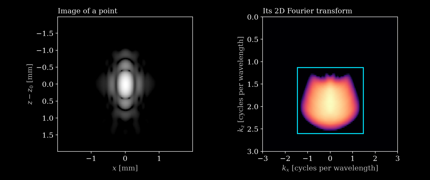
The measured spectrum fills the predicted region, with its outer edges faded by the smooth aperture. The cyan box is the bounding box from aliasing_limits. Only its width along each axis matters for the pitch.

3. Pitch limits

A grid with pitch \(d\) repeats the spectrum every \(1/d\), so each side of the box has to fit in one period. With \(k_\mathrm{lo}\) and \(k_\mathrm{hi}\) the edges of the box along each axis, \(\lambda_\mathrm{min} = c / (f_c + B/2)\) the shortest wavelength in the band, and \(B\) the bandwidth:

Axis	Limit	Approximately
Lateral	\(d_x \le 1 / (k_{x,\mathrm{hi}} - k_{x,\mathrm{lo}})\)	\(\lambda_\mathrm{min} F / 2\) for equal transmit and receive apertures
Axial, RF	\(d_z \le 1 / (2 k_{z,\mathrm{hi}})\)	\(\lambda_\mathrm{min} / 4\)
Axial, IQ	\(d_z \le 1 / (k_{z,\mathrm{hi}} - k_{z,\mathrm{lo}})\)	\(c / (2B)\) on axis

An RF image is real, so axially its mirrored band counts too. Laterally that band sits at the opposite \(k_z\), so RF and IQ have the same limit.

acquisitions = {
    "One plane wave, F=2": ([0.0], 2.0),
    "One plane wave, F=1": ([0.0], 1.0),
    "Compounded ±25°, F=1": (steering, 1.0),
    "Compounded ±25°, F=0.5": (steering, 0.5),
}

print(f"{'Largest pitch, in wavelengths':<30}{'Lateral':>9}{'Axial RF':>10}{'Axial IQ':>10}")
for name, (angles, f) in acquisitions.items():
    iq, rf = limits_for(angles, f, iq=True), limits_for(angles, f, iq=False)
    print(
        f"{name:<30}{iq['dx_max'] / wavelength:>9.2f}"
        f"{rf['dz_max'] / wavelength:>10.2f}{iq['dz_max'] / wavelength:>10.2f}"
    )

Largest pitch, in wavelengths   Lateral  Axial RF  Axial IQ
One plane wave, F=2                1.59      0.19      0.82
One plane wave, F=1                0.86      0.19      0.78
Compounded ±25°, F=1               0.44      0.19      0.75
Compounded ±25°, F=0.5             0.34      0.19      0.68

So \(\lambda/2\) can be too coarse, as for RF and the compounded acquisitions, or needlessly fine, as for the lateral pitch of a single plane wave.

4. Aliasing on the grid

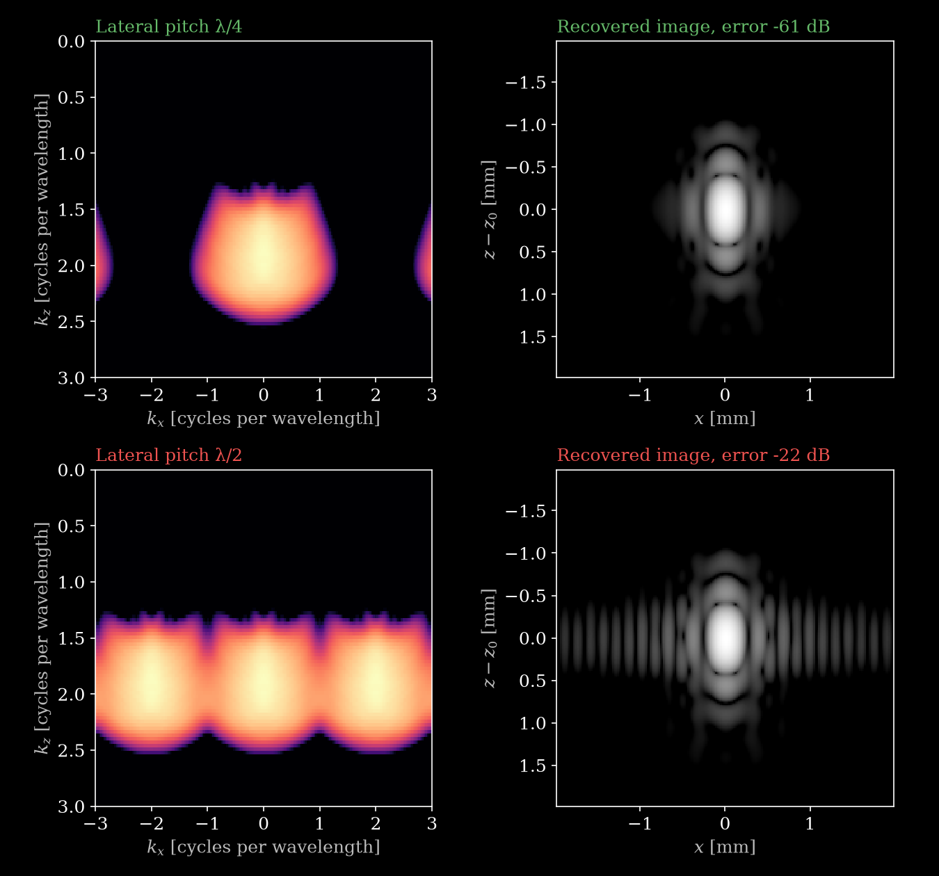
Delay-and-sum computes each pixel independently, with no anti-aliasing filter, so a coarser grid samples the same image at fewer points, and frequencies beyond the limit fold back instead of being smoothed away. We can therefore mimic a coarser grid by keeping every \(M\)-th row or column of pixels in the reference image.

In the examples below, we recover the image with ideal band-limited interpolation and report the error energy relative to the reference image.

First the lateral pitch of the compounded acquisition, which has a limit of \(0.34\lambda\). We compare a pitch below the limit, \(\lambda/4\), with one above it, \(\lambda/2\):

def subsample_and_recover(image, axis, step, center=0.0):
    """Keep every step-th row (axis=0) or column (axis=1), recover by band-limiting.

    Returns the sampled image and the recovered image. `center` is the middle of the kept
    period in cycles per wavelength.
    """
    sampled = np.zeros_like(image)
    keep = [slice(None), slice(None)]
    keep[axis] = slice(None, None, step)
    sampled[tuple(keep)] = step * image[tuple(keep)]

    k = np.fft.fftfreq(n_grid, fine_pitch) * wavelength
    half_period = wavelength / (2 * step * fine_pitch)
    gain = np.abs(k - center) <= half_period
    gain = gain[:, None] if axis == 0 else gain[None, :]
    recovered = np.fft.ifft2(np.fft.fft2(sampled) * gain)
    return sampled, recovered.real if np.isrealobj(image) else recovered


def error_db(recovered, image):
    return 20 * np.log10(np.linalg.norm(recovered - image) / np.linalg.norm(image))


def compare(rows, filename, ylim=(3, 0)):
    """One row per (title, image, axis, step, center, color): spectrum, then recovered image."""
    fig, axes = plt.subplots(len(rows), 2, figsize=(9, 4.2 * len(rows)))
    for ax_row, (title, image, axis, step, center, color) in zip(axes, rows):
        sampled, recovered = subsample_and_recover(image, axis, step, center)
        show_spectrum(ax_row[0], sampled, ylim=ylim)
        ax_row[0].set_title(title, loc="left", color=color)
        show_image(ax_row[1], recovered, reference=envelope(image).max())
        error = error_db(recovered, image)
        ax_row[1].set_title(f"Recovered image, error {error:.0f} dB", loc="left", color=color)
    plt.tight_layout()
    plt.savefig(filename, dpi=150)
    plt.close()


compare(
    [
        ("Lateral pitch λ/4", compounded, 1, 4, 0.0, GREEN),
        ("Lateral pitch λ/2", compounded, 1, 8, 0.0, RED),
    ],
    "kspace_lateral_aliasing.png",
)

Next, one plane wave at \(F = 1\) with an axial pitch of \(\lambda/2\), as IQ and as RF:

single_angle = [0.0]
single_iq = point_target_image(single_angle, 1.0, iq=True)
single_rf = point_target_image(single_angle, 1.0, iq=False)
kz_lo, kz_hi = limits_for(single_angle, 1.0, iq=True)["kz_range"]
band_center = (kz_lo + kz_hi) / 2 * wavelength

compare(
    [
        ("IQ, axial pitch λ/2", single_iq, 0, 8, band_center, GREEN),
        ("RF, axial pitch λ/2", single_rf, 0, 8, 0.0, RED),
    ],
    "kspace_axial_aliasing.png",
    ylim=(3, -3),
)

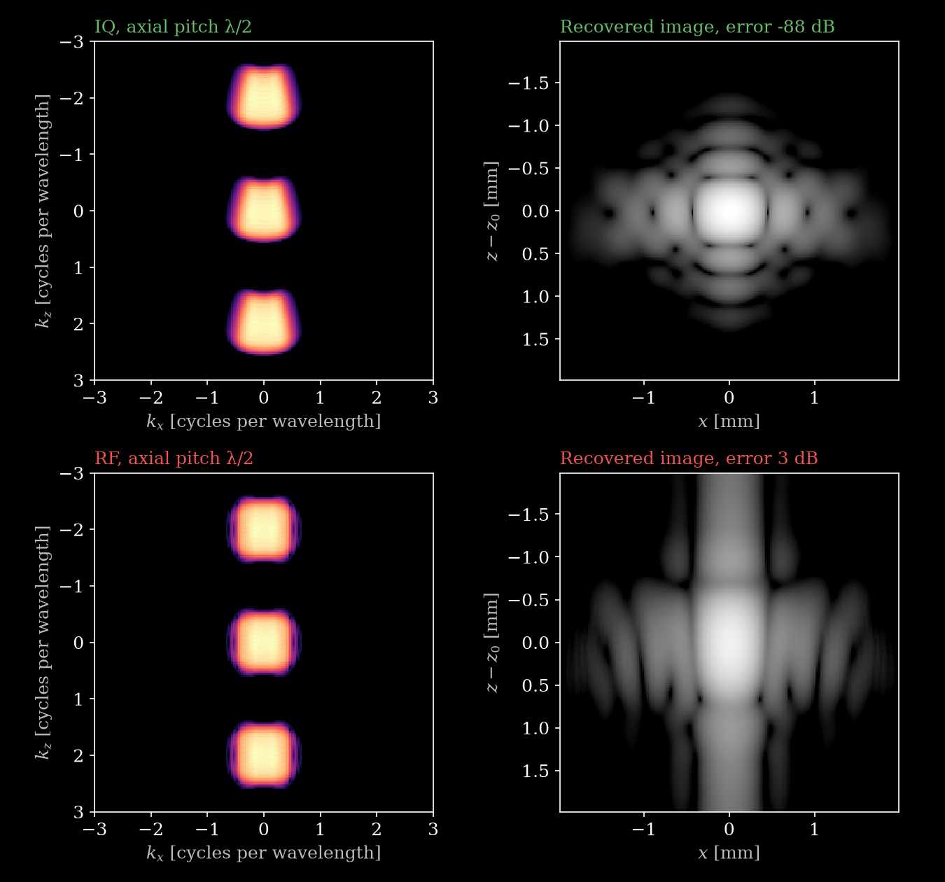
The two spectra look alike, but each RF lobe is the band and its mirror stacked on top of each other, which is why it looks symmetric. Only the IQ image can be recovered.

5. In zea

Parameters checks a cartesian grid against these limits whenever it computes the grid, and warns if the pitch is too large. You can also call the check directly:

coarse = make_parameters(
    steering,
    f_number=f_number,
    grid_size_x=int(2 * half_extent / (wavelength / 2)) + 1,
)
coarse.check_for_aliasing(bandwidth=bandwidth);

zea: WARNING Lateral grid pitch 154.0 um exceeds 104.9 um (lambda_min = 236.9 um, x of the transmit directions in [-0.423, 0.423], sin(theta_r) = +-0.707, element directivity sin(theta) <= 0.928). Consider increasing grid_size_x to 95 or more (for an automatically sized grid, raise pixels_per_wavelength), or narrowing the apertures (f_number / transmit steering) so the data stays inside the grid's lateral band.

The parameters cannot tell two things, so those are up to you:

• RF or IQ. The check assumes IQ, the output of the default pipeline. If you beamform RF, call check_for_aliasing(demodulated=False).

• Bandwidth. Set bandwidth if you know it. Otherwise the check assumes probe_bandwidth_percent of the center frequency, 100% by default, which gives an axial IQ limit close to \(\lambda/2\).

The limits come from a simple model, so leave some margin:

• Hard apertures leak. The default f-number mask and the discrete element positions put faint energy outside the box.

• The edges are soft. Some energy spills just past the box, especially at high f-numbers where the box is narrow, so the error does not drop to zero exactly at the limit.