Autoencoder for ultrasound images

In this notebook, we demonstrate how to use the TAESD tiny autoencoder model for ultrasound images using the zea toolbox. We’ll encode and decode images, visualize the results, and try a simple experiment: interpolating (traveling) in the latent space between two images and animating the result. Note that this model was trained purely on image data, and not finetuned on ultrasound data.

   

‼️ Important: This notebook is optimized for GPU/TPU. Code execution on a CPU may be very slow.

If you are running in Colab, please enable a hardware accelerator via:

Runtime → Change runtime type → Hardware accelerator → GPU/TPU 🚀.

%%capture
%pip install zea

import os

os.environ["KERAS_BACKEND"] = "tensorflow"
os.environ["TF_CPP_MIN_LOG_LEVEL"] = "3"

import matplotlib.pyplot as plt
import numpy as np
from keras import ops
from matplotlib import animation


import zea
from zea import init_device, Dataloader
from zea.models.taesd import TinyAutoencoder
from zea.visualize import plot_image_grid, set_mpl_style

zea: Using backend 'tensorflow'

We will work with the GPU if available, and initialize using init_device to pick the best available device. Also, (optionally), we will set the matplotlib style for plotting.

init_device(verbose=False)
set_mpl_style()

Load data

We load a small batch from the CAMUS validation dataset hosted on Hugging Face Hub.

n_imgs = 4
val_dataset = Dataloader(
    "hf://zeahub/camus-sample/val",
    key="data/image_polar/values",
    batch_size=n_imgs,
    shuffle=True,
    image_size=[256, 256],
    resize_type="resize",
    image_range=[-60, 0],
    normalization_range=[-1, 1],
    seed=42,
)
batch = next(iter(val_dataset))

zea: WARNING Key 'data/image_polar/values' with 3 dimensions does not match any field of the zea file spec, so the axis that stores frames is unknown. Assuming axis 0.

Load TAESD Model

We use the built-in TAESD model from zea.

model = TinyAutoencoder.from_preset("taesdxl")

Encode and Decode

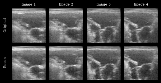
We encode and decode the images using the autoencoder. TAESD expects grayscale or RGB, so we keep the input as is.

recon = model(batch)
mse = ops.convert_to_numpy(ops.mean((recon - batch) ** 2))
print("MSE (reconstruction):", mse)

MSE (reconstruction): 0.009776436

Visualization

We plot the original images and reconstructions for comparison.

imgs = [zea.display.to_8bit(batch[i], (-1, 1), pillow=False) for i in range(n_imgs)] + [
    zea.display.to_8bit(recon[i], (-1, 1), pillow=False) for i in range(n_imgs)
]

titles = [f"Image {i + 1}" for i in range(n_imgs)]

fig, _ = plot_image_grid(
    imgs,
    ncols=n_imgs,
    remove_axis=False,
    figsize=(n_imgs * 2, 3),
)
for i, ax in enumerate(fig.axes[:n_imgs]):
    ax.set_title(titles[i], fontsize=8)
fig.axes[0].set_ylabel("Original", fontsize=8)
fig.axes[n_imgs].set_ylabel("Recon", fontsize=8)
plt.show()

Latent Space Interpolation

Let’s pick two images, encode them, and interpolate between their latent representations. We’ll decode each interpolated latent and animate the result to visualize a smooth transition between two ultrasound images. Again, note that this model was trained on natural images only, and improved results are expected with a finetuned model on ultrasound data (to be added!).

# Pick two images to interpolate between
img_a = batch[0][None, ...]
img_b = batch[2][None, ...]

latent_a = model.encode(img_a)
latent_b = model.encode(img_b)

n_steps = 12
alphas = np.linspace(0, 1, n_steps)
frames = []
for alpha in alphas:
    latent_interp = (1 - alpha) * latent_a + alpha * latent_b
    recon_interp = model.decode(latent_interp)
    frames.append(zea.display.to_8bit(recon_interp[0], (-1, 1), pillow=False))

fig, ax = plt.subplots(figsize=(5, 4), dpi=50)
im = ax.imshow(frames[0], cmap="gray", vmin=0, vmax=255)
ax.axis("off")


def animate(i):
    im.set_data(frames[i])
    return [im]


ani = animation.FuncAnimation(fig, animate, frames=len(frames), interval=100, blit=True)
plt.close(fig)
ani.save("latent_interpolation.gif")

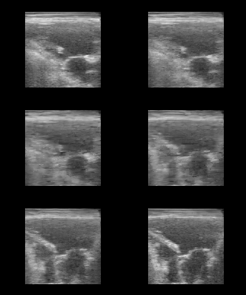
You should see a smooth morphing between two ultrasound images, demonstrating the structure of the TAESD latent space.